Why LSTMs Work: The One Line That Makes Long-Range Memory Possible
On this page
Give a plain recurrent neural network a sentence and ask it to connect a pronoun to an antecedent forty words back, and it will fail. Not because it lacks the capacity — an RNN is Turing-complete in the limit — but because the training signal never arrives. By the time the gradient has travelled forty steps backwards, it has been multiplied down to roughly the size of floating-point noise.
The Long Short-Term Memory cell fixes this. It is often taught as a bag of gates to memorise, which makes it look arbitrary and fussy. It isn't. Every part of the architecture follows from one diagnosis and one fix, and once you see the fix you'll recognise it in ResNets, in Transformers, and in most things that have worked since.
The problem: gradients die exponentially
A recurrent network keeps a hidden state that it updates with the same function at every step:
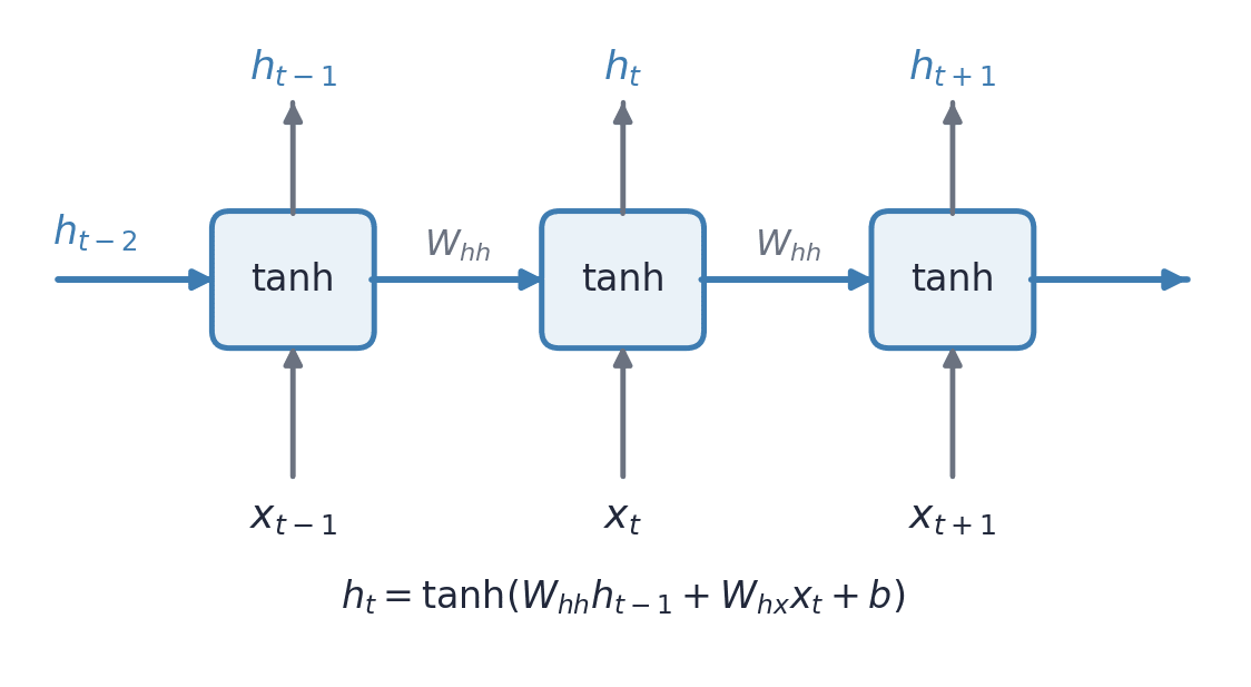
Unrolling this through time gives you a network as deep as your sequence is long, with every layer sharing the same weights. That depth is where the power comes from, and also the pathology.
When you backpropagate, the gradient from step to some earlier step has to pass through a product of Jacobians:
Take norms and you get a bound on each factor: the spectral norm of times the largest attainable activation derivative. Call that product . Then
That exponent is the whole story. If \eta < 1 the gradient vanishes; if it explodes. And \eta < 1 is the overwhelmingly common case, because both nonlinearities have hard ceilings on their derivatives — , and everywhere. A saturated unit, which is exactly what a unit that has committed to a decision looks like, has a derivative near zero.
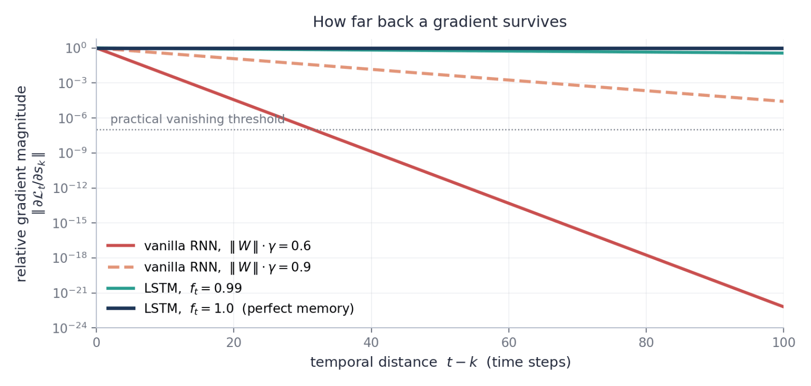
With , a signal thirty steps back arrives attenuated by a factor of about .
The two failure modes are not symmetric, and this is worth dwelling on. Exploding gradients are loud — the loss spikes, you get NaNs, and a norm clip fixes it in one line. Vanishing gradients are silent. The model trains. The loss goes down. Nothing looks wrong. It has simply learned only the short-range structure, because the long-range structure never produced a usable learning signal. A language model that can't link a pronoun to its antecedent still produces perfectly fluent local text, and you only find out in careful evaluation.
What a fix has to look like
The decay has two causes: repeated multiplication by a fixed weight matrix, and repeated multiplication by a saturating activation derivative. So any fix has to provide a route through time where neither appears.
Two more requirements, and these are the ones people skip:
- The per-step multiplier on that route should be close to 1.
- It should be learned and input-dependent, so the network decides for itself what deserves to persist and for how long. A fixed decay constant would be useless — you'd be hard-coding a single time horizon for every piece of information the model ever sees.
The LSTM cell
The structural move is to separate what the cell remembers from what the cell reveals.
Where a vanilla RNN has one state vector, an LSTM has two. The cell state is the memory: updated additively, never squashed on its way from one step to the next. The hidden state is the output: a bounded, filtered view of the memory that the rest of the network gets to see. Three gates — vectors in produced by sigmoid units — control writing, erasure and exposure.
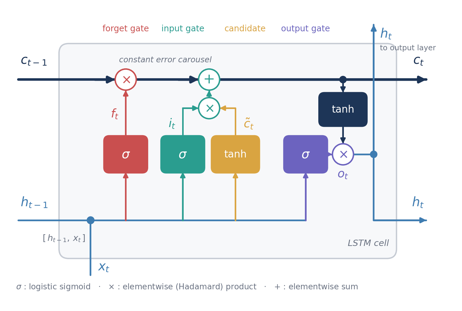
Here is the whole forward pass:
Six lines. Reading them in order:
The forget gate decides, per memory slot, what fraction of the existing contents survives. An element near 1 preserves that slot; near 0 erases it. Because it's a function of the current input and previous output, the decision is made on the fly — a model reading a sentence boundary can clear the slots holding the previous subject while leaving discourse-level context untouched.
The input gate and candidate split writing into two decisions: how much to write () and what to write (). This factoring matters. The network can compute a confident, large-magnitude candidate and still decline to store it, or store a little of a tentative one. An unfactored update would have to encode magnitude and admissibility in the same numbers.
The output gate decides how much of the memory to reveal right now. The tanh bounds the exposed value regardless of how large the accumulated memory has grown; then selects which slots are relevant. This separation is easy to overlook and is doing real work — a fact can sit in for a hundred steps with near zero, invisible to every downstream layer and to the gates of the next step, then be released the moment it becomes relevant.
The one line that matters
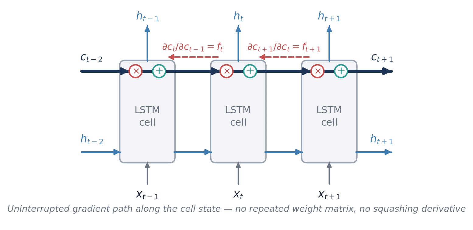
Note what this is not. It is not a matrix product, and it is not passed through an activation function. The old memory is scaled elementwise and the new content is added.
Differentiate it with respect to the previous cell state, holding fixed — that is, along the direct route through the memory lane:
Compare that with the RNN Jacobian above. There, each step contributed . Here, each step contributes a diagonal matrix of gate values and nothing else — no weight matrix, no activation derivative. Composing over a span:
Hochreiter and Schmidhuber called this the constant error carousel: an unobstructed path along which error circulates essentially undiminished.
How long is "long"?
The product form turns a qualitative claim into arithmetic. If a slot holds its forget gate at a constant , the memory decays geometrically with a well-defined half-life:
| Forget gate | Half-life |
|---|---|
| 0.5 | 1 step |
| 0.9 | 7 steps |
| 0.99 | 69 steps |
| 0.999 | 693 steps |
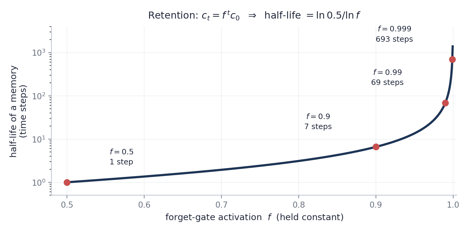
The sensitivity near is dramatic — a change of one part in a thousand moves the memory horizon by two orders of magnitude. And because the gate is computed per element, different units in the same layer settle on completely different time constants. Some become fast-decaying detectors of local structure; others become near-lossless registers holding a fact for hundreds of steps. Nobody designs this decomposition. The network discovers it, and which units specialise in what depends on the task.
A worked example you can check by hand
Take the smallest possible cell, , so every vector is a scalar. An important signal arrives at and must be reported at , with an irrelevant step in between.
| Step | |||||||
|---|---|---|---|---|---|---|---|
| 1 — store | 1.0 | 0.95 | 0.90 | 0.80 | 0.60 | 0.7200 | 0.3701 |
| 2 — hold | 0.0 | 0.98 | 0.05 | −0.30 | 0.20 | 0.6906 | 0.1197 |
| 3 — recall | 0.0 | 0.99 | 0.02 | 0.10 | 0.90 | 0.6857 | 0.5357 |
Read the two right-hand columns against each other, because that contrast is the whole point.
At , the input gate is open and 0.72 goes into memory. At nothing relevant arrives: the input gate nearly closes, the forget gate stays open, and the memory persists at 0.6906 — 95.9% of what was stored. But the output gate closes to 0.20 and the hidden state falls to 0.1197, a value close enough to zero that any downstream layer reads it as "nothing here." At the output gate opens and the stored value is released.
The hidden state went 0.37 → 0.12 → 0.54 while the memory went 0.720 → 0.691 → 0.686. An observer with access only to would conclude the information was lost at and mysteriously reappeared at . This is impossible in an architecture with a single state vector.
The gradient story is just as concrete. Along the carousel, sensitivity of the final memory to the stored value is — a 3% attenuation over two steps. A vanilla RNN with a realistic per-step factor of 0.5 delivers , a 75% loss over the same span.
The caveat nobody mentions
Most explanations stop at and let you believe the vanishing gradient problem is solved. It isn't, and the equation above is a partial derivative.
The total derivative also contains indirect terms, because influences through , and feeds all four gates at the next step. Those indirect paths do involve weight matrices and saturating derivatives, and they do decay.
The honest claim is narrower and still sufficient: the LSTM provides one path that does not vanish, and gradient descent needs only one. Exploding gradients, meanwhile, are not addressed by this construction at all — you still need norm clipping.
One line of code worth more than most tuning
If all biases start at zero, then at initialisation , giving every memory a half-life of exactly one step. Your network starts in the regime where long-range gradients are already dead and has to climb out of it before it can learn anything long-range — a chicken-and-egg problem.
So bias the forget gate open from the start:
1 2 3 4 5 6# after constructing the layer n = lstm.hidden_size for name, param in lstm.named_parameters(): if "bias" in name: # PyTorch layout: [i | f | g | o] param.data[n:2*n].fill_(1.0)
, which is a half-life of about 2 steps instead of 1 — and, more importantly, a starting point from which the gate can easily learn its way up to 0.99. Gers and colleagues recommended this in 2000; Jozefowicz and colleagues confirmed it at scale in 2015. It costs nothing and frequently makes the difference between a model that captures long dependencies and one that doesn't.
Are LSTMs obsolete?
Transformers displaced them from the centre of the field, and the reason is parallelism rather than accuracy. An LSTM must compute before : the recurrence is inherently sequential, so training time scales with sequence length no matter how much hardware you throw at it. Self-attention compares every position with every other in one parallel operation. Its cost is quadratic in length rather than linear, but that quadratic work parallelises, and on modern accelerators parallel quadratic beats sequential linear by a wide margin.
That said, treating LSTMs as obsolete is a mistake. They remain the right choice for:
- Streaming and real-time inference. Fixed-size state, constant time and memory per step. A Transformer's per-step cost grows with the history.
- Very long sequences under memory pressure. Linear rather than quadratic scaling in length.
- Small-data regimes. The recurrent inductive bias — recent past matters most, same update everywhere — is a real prior. Transformers must learn positional structure from data, and with limited data they often don't.
- Embedded and edge deployment. Constant memory per step and small parameter counts suit microcontrollers and on-device sensor processing.
And the central idea outlived the architecture anyway. The residual connection that makes deep networks trainable is the same additive-path argument, moved from the time axis to the depth axis. The recent family of state-space models revisits the gated-accumulator formulation with parallelisable scans. The constant error carousel turned out to be a far more durable contribution than the cell that introduced it.
If you take one thing away: when a gradient has to travel a long way, give it a path with a derivative of one and let the network decide when to open it.